Gerrit de Rooij's public domain codes

All codes below are in Fortran, and developed by me for use in my own research. The comments in the source codes identify any algorithms or ideas adopted from the literature and give full references to the relevant papers and websites. Unless stated otherwise, I did not use code from others so the copyright rests solely with UFZ.

When you use any of the material on this website, please acknowledge me as the author of the material.

Rainfall generator

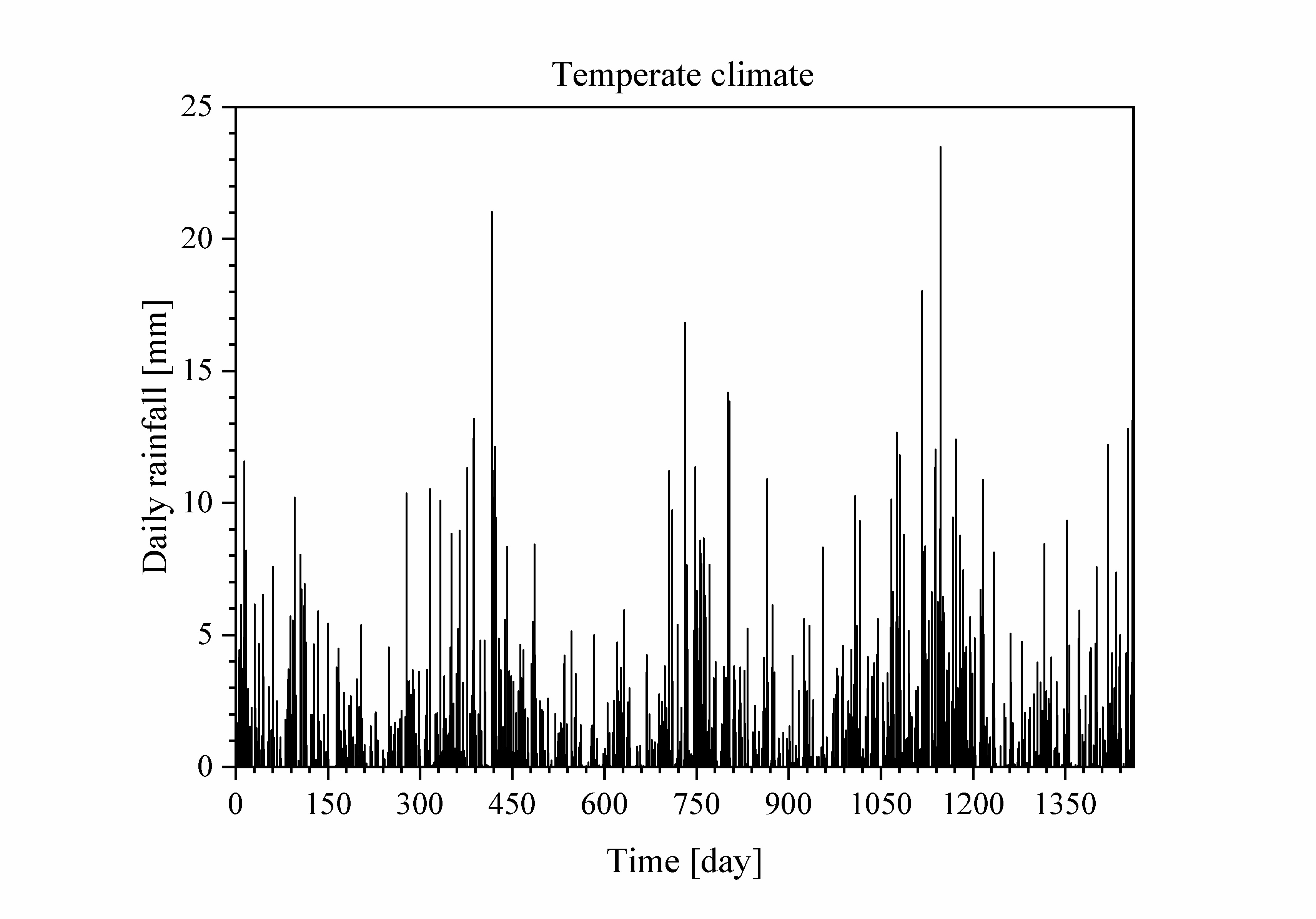
Main features

This Fortran 90 program simulates rainfall according to one of several Bartlett-Lewis-type models described in Pham et al. (2013). Of these, the most basic is left out. The others are the model described by Rodriguez-Iturbe et al. (1988) or modifications thereof. One of these modifications is Onof et al.'s (2013) suggestion to truncate the gamma-distribution of eta (see below). Another is to replace the exponential distribution of the rainfall rate in a rainfall cell by a gamma distribution. This leads to four model configurations (abbreviations according to Pham et al., 2013):

1) MBL: Bartlett-Lewis with the parameters characterizing a storm (pdf of storm duration and pdf of cell arrival times) related to a gamma-distributed parameter eta. The rainfall rate in a rain cell has an exponential distribution. This is the Modified Bartlett-Lewis model, introduced by Rodriguez-Iturbe et al. (1988).

2) TBL: As MBL, but with a truncated gamma distribution for eta (Truncated Bartlett-Lewis).

3) MBLG: As MBL, but with the rainfall rate per cell having a gamma distribution.

4) TBLG: As TBL, but with the rainfall rate per cell having a gamma distribution.

Leap years are automatically taken into consideration. The code assumes that the first day of the period for which the rainfall record is to be generated is January 1st of a year immediately following a leap year. This feature simplifies the generation of rainfall records spanning multiple decades or even centuries.

For very long rainfall series using the untruncated gamma distribution can lead to physically unrealistic rainfall amounts because for small values of eta, the moments of the gamma distribution are unbounded for values of alpha < 4 (Onof et al., 2103). Excessively small values of eta can be avoided by simply not permitting values below a threshold epsilon, which is the rationale for TBL and TBLG. Pham et al. (2013) found that MBL outperformed the other models, but still TBL might be a good choice. For that reason, MBL and MBLG are not explicitly included in the input. To run an MBL- or MBLG-type model, the parameter lower_eta, which gives the lower threshold for eta, needs to be set to zero in the input file for each period for which the parameters are given.

The code requires the model parameters for arbitrary periods of time in which a year is subdivided (usually for each month). Storms are generated for a given period until the starting time of a storm is beyond that period. This starting time is not discarded, but it serves as the starting time of the first storm in the period in which it occurs. The parameters of that storm are generated using the pdfs for the period in which it occurs, not the period in which it was generated. Subsequent storms are generated using the parameters of that period. Rain cells in a storm are generated until a rain cell has a starting time that exceeds the time at which the storm ends. This latest cell is discarded. Rain cells may overlap, creating irregular rainfall rates over time.

The resulting rainfall from individual cells is used to create a time line of rainfall rates (including zero, for dry spells) that gives a continuous record of the rainfall rate as a function of time. This record is processed to provide hourly, daily, monthly, and annual sums. The full timeline and the hourly sums are only written to output files if the input file stipulates it. Daily, monthly, and annual sums are always written to output files. The annual and monthly averages and their standard deviations are also written to an output file.

References

Kim, D., F. Olivera, H. Cho, and S.A. Socolofsky. 2013. Regionalization of the modified Bartlett-Lewis rectangular pulse stochastic rainfall model. Terr. Atmos. Ocean. Sci. 24:421-436. Doi:10.3319/TAO.2012.11.12.01(Hy).

Onof, C., R.E. Chandler, A. Kakou, P. Northrop, H.S. Wheater, and V. Isham. 2000. Rainfall modelling using Poisson-cluster processes: a review of developments. Stochastic Environmental Research and Risk Assessment 14:384-411.

Onof, C., W.J. Vanhaute, T. Meca-Figueras, J. Kaczmarska, R. Chandler, L. Hege, S. Vanderberghe, P. Willems, and N.E.C. Verhoest. 2013. A truncated random parameter version of the Bartlett-Lewis model. Unpublished communication.

Pham, M.T., W.J. Vanhaute, S. Vanderberghe, B. De Baets, and N.E.C. Verhoest. 2013. An assessment of the ability of Bartlett-Lewis type of rainfall models to reproduce drought statistics. Hydrol. Earth Syst. Sci. 17:5167-5183. www.hydrol-earth-syst-sci.net/17/5167/2013/. Doi:10.5194/hess-17-5167-2013.

Rodriguez-Iturbe, I., D.R. Cox, and V. Isham. 1988. A point process model for rainfall: further developments. Proc. R. Soc. Lond. A 417:283-298.

Xi, B., K.M. Tan, and C. Liu. 2013. Logarithmic transformation-based gamma random number generators. J. Statistical Software 55 (4):1-17.

Temperature and evapotranspiration generator

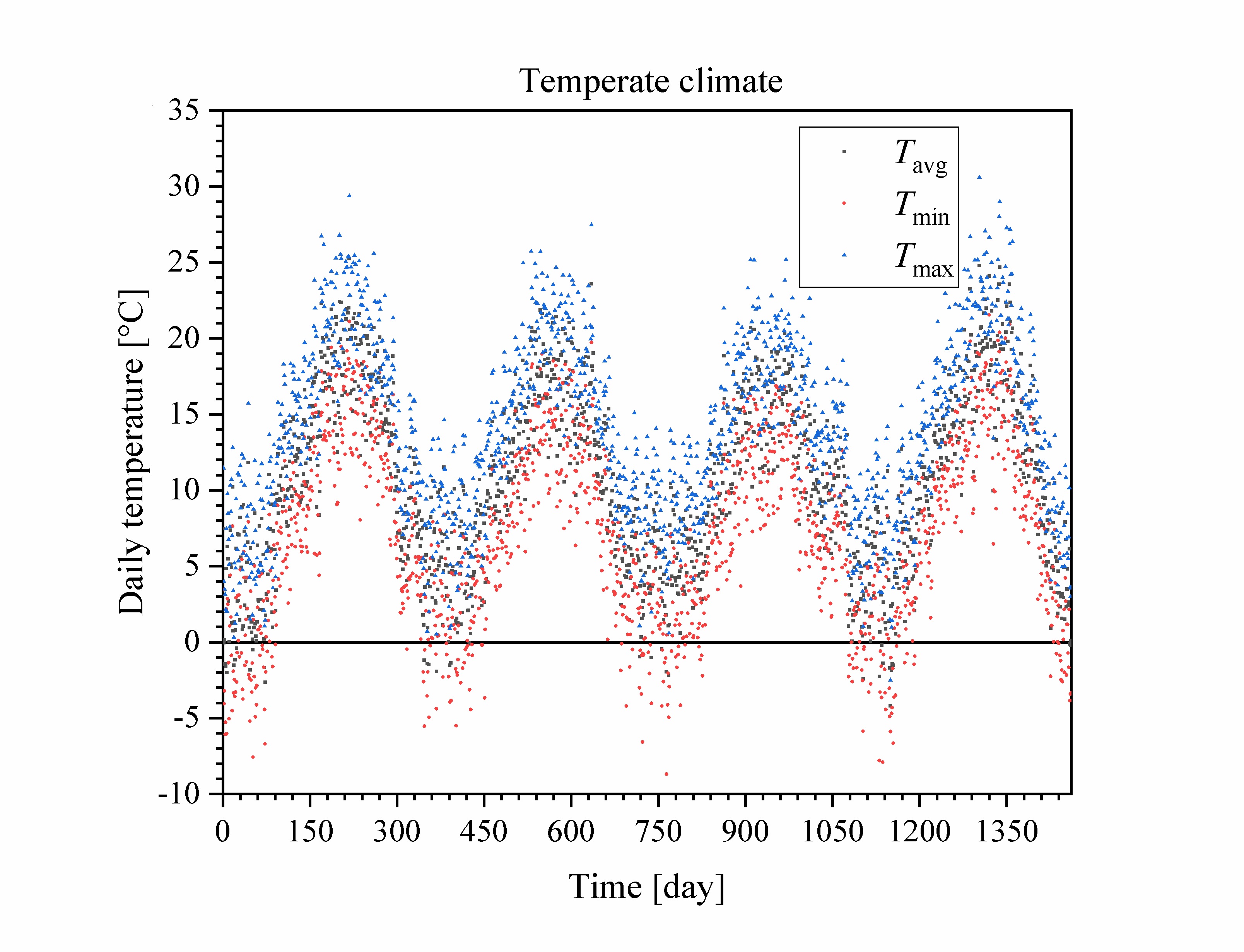
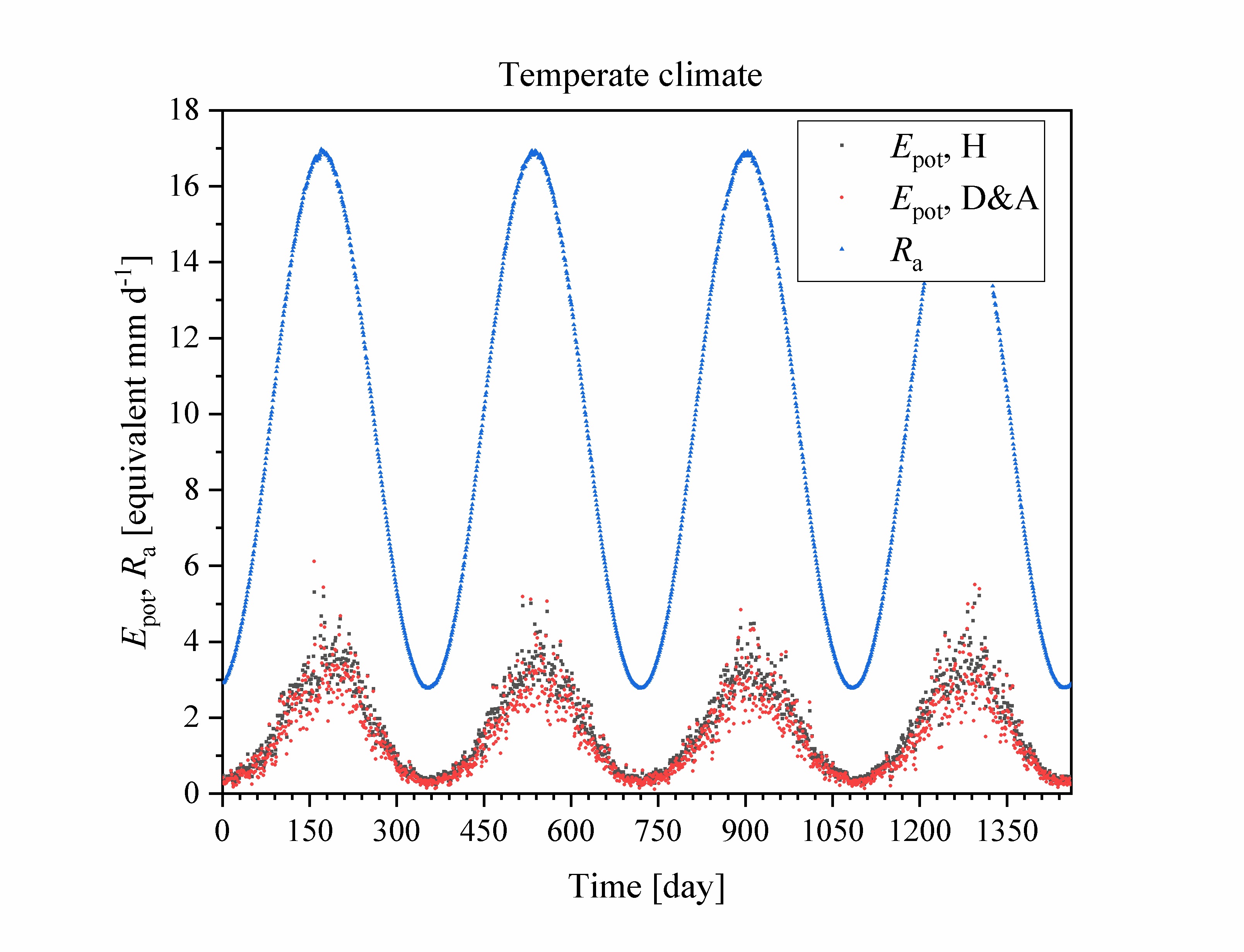
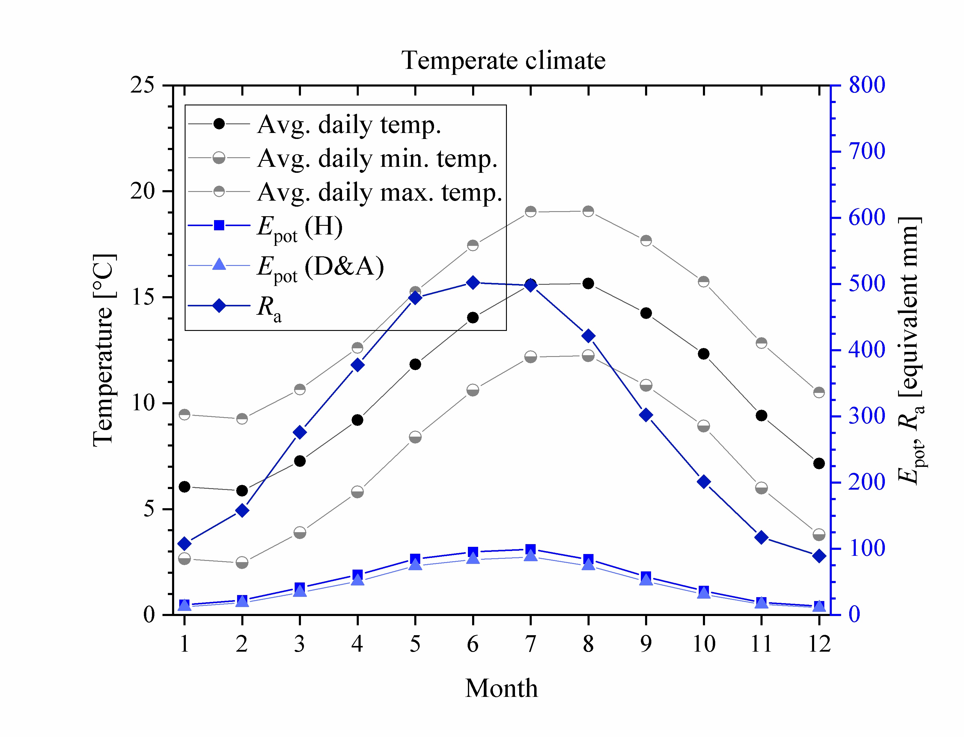
Main features

The temperature generator produces daily values for the average, minimum and maximum temperature. It also assigns to each day a probability that that day is overcast, and then determines randomly if each day is cloudy.

The average daily temperature is assumed to have a sinusoidal trend over the year. To allow inter-annual variation, the amplitude and the mean of the sinusoidal signal are independently normally distributed. The de-trended daily mean temperatures are first order autoregressive with zero mean and independent, normally distributed shocks.

The range between the daily minimum and maximum temperatures is also assumed to be random and identically independently distributed, but with a lognormal distribution. The minimum and maximum daily temperatures are generated by superimposing lognormally distributed fluctuations on the daily mean temperature.

On cloudy days, the amplitude of the annual trend and the standard deviation of the daily fluctuations around the mean are reduced.

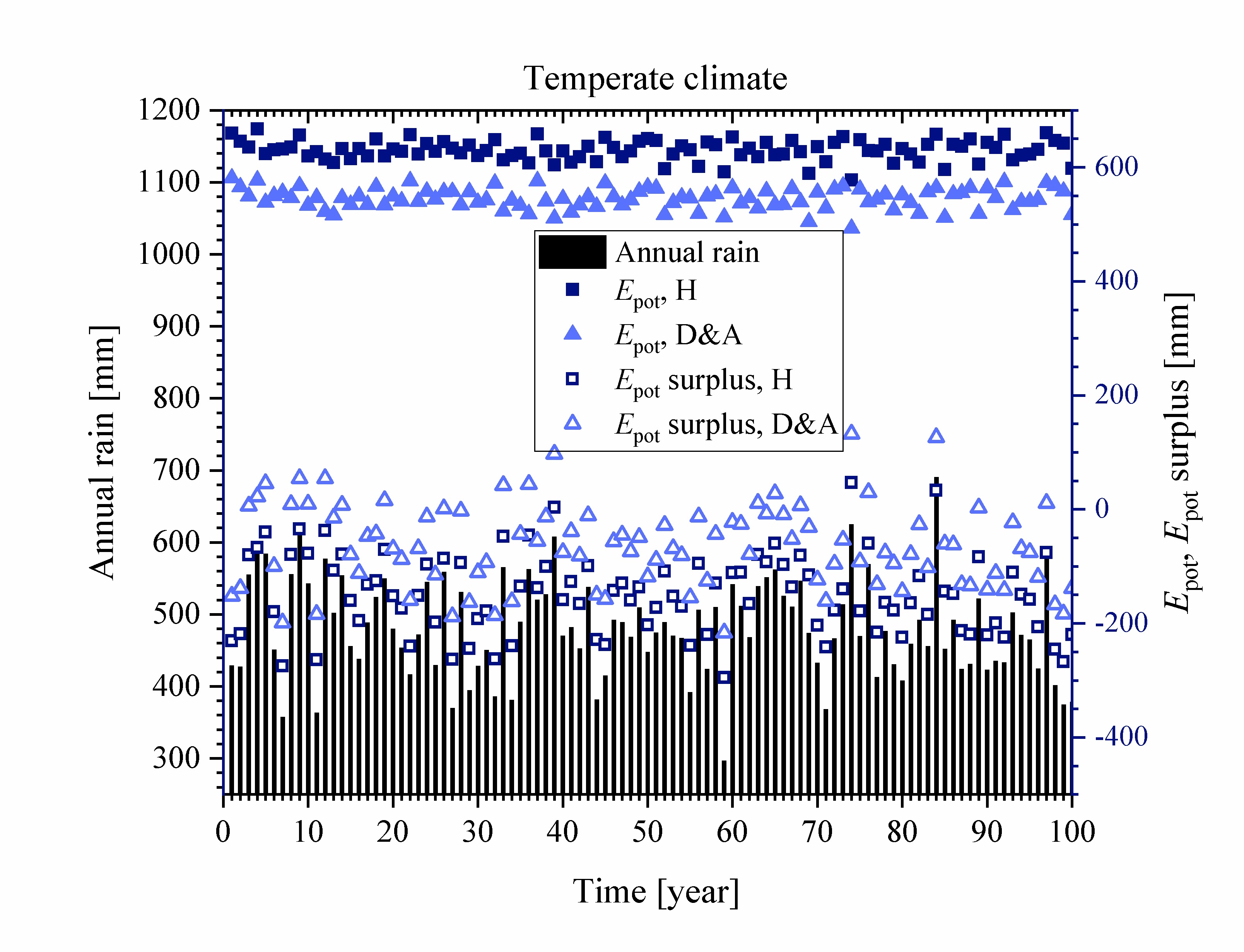
The daily potential evapotranspiration can be estimated from the daily temperature extremes and the extraterrestrial radiation according to Hargreaves (1994) equation. A modified version developed by Droogers and Allen (2002) also uses the monthly rainfall. In the code I replaced the monthly rainfall by the rainfall sum in the 30-day time window centred around the day of interest.

The code generates daily records of the mean, minimum, and maximum temperature, of the extraterrestrial radiation, of the cloudiness (a day can be clear or overcast), and of the potential evapotranspiration according to the two models referenced above. It also provides monthly and annual averages of all weather characteristics except rainfall.

The code takes input from TempEpot.IN, Daily_Rain.OUT, Monthly_Rain.OUT, and Annual_Rain.OUT (the latter three come from the rainfall generator).

References

Droogers, P., and R.G. Allen. 2002 Estimating reference evapotranspiration under inaccurate data conditions. Irrigation and Drainage Systems 16:33-45.

Hargreaves, G. H. Defining and using reference evapotranspiration. J. Irrigation and Drainage Engineering 120:1132-1139.

Groundwater model

Analytical solution of groundwater flow in a rectangular aquifer (strip aquifer) between a watershed and a canal or ditch

For aquifers along long canals or ditches, the flow can be assumed to be perpendicular to the canal, leading to parallel flow in the aquifer. This leads to a two-dimensional flow system. By invoking the Dupuit-Forchheimer assumptions and requiring that the variation in aquifer thickness is negligible, the flow becomes strictly horizontal and vertically uniform, reducing the system to a one-dimensional problem. This allows the flow equation (Boussinesq-equation) to be linearized, which gives considerable flexibility in the initial and boundary conditions and the external forcing for which an analytical solution is still possible.

The linearized Boussinesq-equation was solved for a strip aquifer between a zero-flux boundary and a prescribed head boundary. Uniform recharge/extraction is allowed. The aquifer may exchange water with a deeper aquifer through a leaky aquitard with constant and uniform resistance. The hydraulic head in the deeper aquifer must be uniform and constant. The recharge/extraction must be uniform but may vary arbitrarily in time. The prescribed head may also vary arbitrarily. The initial hydraulic head can vary arbitrarily over the length of the aquifer.

The derivation of the solution to this problem can be downloaded below. The steady-state solution was derived as well.  Both solutions consist of an infinite sum. A Fortran90 code was developed to implement the solution. The code, the executable, and a set of example input files can also be downloaded below. 

On input, the six aquifer parameters (length, depth, conductivity, storativity, and two parameters describing the exchange with the deeper aquifer) are required. The convergence of the infinite sum is checked each time a user-prescribed number of terms has been calculated and is terminated if a user-prescribed tolerance criterion is met. To avoid excessively long run times, the user also needs to specify the maximum number of terms of the sum that will be evaluated. The number of locations and times for which the hydraulic head should be computed should also be provided. Finally, the number of locations for which the initial hydraulic head is provided, the number of times for which the prescribed hydraulic head is given, and the number of times for which recharge/extraction is given need also to be given on input. All this information is provided in Dupuitflow.IN.

File H1.In gives the times for which the prescribed head is given and the corresponding values. Hinitial.IN gives the locations where the initial hydraulic head is given, and the values. R.In contains the recharge rates and the time intervals to which they apply. OutputTimes.IN and OutputLocations.IN give the times and locations for which the hydraulic head will be written to output.

Full details about the input and output requirements is given in the heading of the file with the source code (DupuitFlow4.F90). Additional information about some of the output is given in de Rooij (2012, 2013)

References

de Rooij, G.H. 2012. Transient flow between aquifers and surface water: analytically derived field-scale hydraulic heads and fluxes. Hydrol. Earth Syst. Sci. 16:649-669. www.hydrol-earth-syst-sci.net/16/649/2012/. Doi:10.5194/hess-16-649-2012 (open access).

de Rooij, G.H. 2013. Aquifer-scale flow equations as generalized linear reservoir models for strip and circular aquifers: Links between the Darcian and the aquifer scale. Water Resour. Res. 49:8605-8615. Doi:10.1002/2013WR014873.

Disclaimer

The source code, executables, and all other files come without any warranty, including any implied warranty of merchantability or fitness for a particular purpose. Neither the author nor the Helmholtz Zentrum für Umweltforschung – UFZ, GmbH can be held liable for any consequence from the use of the codes and/or files presented here or any modifications thereof.

Weather generator

Example input files for a climate representative of Ukkel (Belgium). See Pham et al. (2013) for the rainfall parameter values.

Example input files for a hypothetical arid climate with two seasons

Groundwater model